
Deep GPVAR: Upgrading DeepAR For Multi-Dimensional Forecasting
Amazon’s hidden forecasting gem


What is the most enjoyable thing when you read a new paper? For me, this is the following:
Imagine a popular model suddenly getting upgraded — with just a few elegant tweaks.
Three years after DeepAR [1], Amazon engineers published its revamped version, known as Deep GPVAR [2] (Deep Gaussian-Process Vector Auto-regressive) or simply GPVAR. Some papers also call it GP-Copula.
This is a much-improved model of the original version. Plus, it’s open-source! In this article, we discuss:
How Deep GPVAR works in depth.
How DeepAR and Deep GPVAR are different.
What problems does Deep GPVAR solve and why it’s better than DeepAR?
A hands-on tutorial on energy demand forecasting.
Find the hands-on project for Deep GPVAR in the AI Projects folder, along with other cool projects!
What is Deep GPVAR?
Deep GPVAR is an autoregressive DL model that leverages low-rank Gaussian Processes to model thousands of time-series jointly, by considering their interdependencies.
Let’s briefly review the advantages of using Deep GPVAR :
Multiple time-series support: The model uses multiple time-series data to learn global characteristics, improving its ability to forecast accurately.
Extra covariates: Deep GPVAR allows extra features (covariates).
Scalability: The model leverages low-rank gaussian distribution to scale training to multiple time series simultaneously.
Multi-dimensional modeling: Compared to other global forecasting models, Deep GPVAR models time series together, rather than individually. This allows for improved forecasting by considering their interdependencies.
The last part is what differentiates Deep GPVAR from DeepAR. We will discuss this more in the next section.
Global Forecasting Mechanics
A global model trained on multiple time series is not a new concept. But why the need for a global model?
At my previous company, where clients were interested in time-series forecasting projects, the main request was something like this:
“We have 10,000 time-series, and we would like to create a single model, instead of 10,000 individual models.”
The time series could represent product sales, option prices, atmospheric pollution, etc. — it doesn't matter. What’s important here is that a company needs a lot of resources to train, evaluate, deploy, and monitor (for concept drift) 10,000 time series in production.
So, that is a good reason. Also, at that time, there was no N-BEATS or Temporal Fusion Transformer.
However, if we are to create a global model, what should it learn? Should the model just learn a clever mapping that conditions each time series based on the input? But, this assumes that time series are independent.
Or should the model learn global temporal patterns that apply to all time series in the dataset?
Interdependencies Of Time Series
Deep GPVAR builds upon DeepAR by seeking a more advanced way to utilize the dependencies between multiple time series for improved forecasting.
For many tasks, this makes sense.
A model that considers time series of a global dataset as independent loses the ability to effectively utilize their relationships in applications such as finance and retail. For instance, risk-minimizing portfolios require a forecast of the covariance of assets, and a probabilistic forecast for different sellers must consider competition and cannibalization effects.
Therefore, a robust global forecasting model cannot assume the underlying time series are independent.
Deep GPVAR is differentiated from DeepAR in two things:
High-dimensional estimation: Deep GPVAR jointly models time series together, factoring in their relationships. For this purpose, the model estimates their covariance matrix using a low-rank Gaussian approximation.
Scaling: Deep GPVAR does not simply normalize each time series, like its predecessor. Instead, the model learns how to scale each time series by transforming them first using Gaussian Copulas.
The following sections describe how these two concepts work in detail.
Low-Rank Gaussian Approximation — Introduction
As we said earlier, one of the best ways to study the relationships of multiple time series is to estimate the covariate matrix.
However, scaling this task for thousands of time series is not easily accomplished — due to memory and numerical stability limitations. Plus, covariance matrix estimation is a time-consuming process — the covariance should be estimated for every time window during training.
To address this issue, the authors simplify the covariance estimation using low-rank approximation.
Let’s start with the basics. Below is the matrix form of a Multivariate normalN∼(μ,Σ) with mean μ ∈ (k,1) and covariance Σ ∈ (k,k)

The problem here is the size of the covariance matrix Σ that is quadratic with respect to N, the number of time series in the dataset.
We can address this challenge using an approximated form, called the low-rank Gaussian approximation. This method has its roots in factor analysis and is closely related to SVD (Singular Value Decomposition).
Instead of computing the full covariance matrix of size (N,N), we can approximate by computing instead:
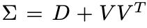
where D ∈ R(N,N) is a diagonal matrix and V ∈ R(N,r).
But why do we represent the covariance matrix using the low-rank format? Because sincer<<N, it is proved that the Gaussian likelihood can be computed using O(Nr² + r³) operations instead of O(N³) (the proof can be found in the paper’s Appendix).
The low-rank normal distribution is part of PyTorch’s distributions module. Feel free to experiment and see how it works:
# multivariate low-rank normal of mean=[0,0], cov_diag=[1,1], cov_factor=[[1],[0]]

# covariance_matrix = cov_diag + cov_factor @ cov_factor.T

m = LowRankMultivariateNormal(torch.zeros(2), torch.tensor([[1.], [0.]]),
torch.ones(2))
m.sample()
#tensor([-0.2102, -0.5429])
Deep GPVAR Architecture
Notation: From now on, all variables in bold are considered either vectors or matrices.
Now that we have seen how low-rank normal approximation works, we delve deeper into Deep GPVAR’s architecture.
First, Deep GPVAR is similar to DeepAR — the model also uses an LSTM network. Let’s assume our dataset contains N time series, indexed from i= [1…N]
At each time step t we have:
An LSTM cell takes as input the target variable
z_t-1of the previous time stept-1for a subset of time series. Also, the LSTM receives the hidden stateh_t-1of the previous time step.The model uses the LSTM to compute its hidden vector
h_t.The hidden vector
h_twill now be used to compute theμ, Σparameters of a multivariate Gaussian distributionN∼(μ,Σ). This is a special kind of normal distribution called Gaussian copula (More about that later).
This process is shown in Figure 1:


At each time step t, Deep GPVAR randomly chooses B << N time-series to implement the low-rank parameterization: On the left, the model chooses from (1,2 and 4) time series and on the right, the model chooses from (1,3 and 4).
The authors in their experiments have configured B = 20. With a dataset containing potentially over N = 1000 time series, the benefit of this approach becomes clear.
There are 3 parameters that our model estimates:
The means
μof the normal distribution.The covariance matrix parameters are
dandvaccording to Equation 2.
They are all calculated from the h_t LSTM hidden vector. Figure 2 shows the low-rank covariance parameters:

Careful with notation:
μ_i,d_i,v_irefer to thei-thtime series in our dataset, wherei ∈ [1..N].
For each time-series i, we create the y_i vector, which concatenates h_iwith e_i — the e_i vector contains the features/covariates of the i-th time series. Hence we have:
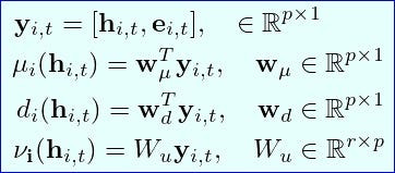
Figure 3 displays a training snapshot for a time step t:

Notice that:
μanddare scalars, whilevis vector. For example,μ = w_μ^T * ywith dimensions(1,p)*(p,1), thereforeμis a scalar.The same LSTM is used for all time series, including the dense layer projections
w_μ,w_d,w_u.
Hence, the neural network parameters w_μ ,w_d ,w_uandy are used to compute the μ and Σ parameters which are shown in Figure 3.
The Gaussian Copula Function
Question: What does the
μandΣparameterize?
They parameterize a special kind of multivariate Gaussian distribution, called Gaussian Copula.
But why does Deep GPVAR needs a Gaussian Copula?
Remember, Deep GPVAR does joint multi-dimensional forecasting, so we cannot use a simple univariate Gaussian, like in DeepAR.
Ok. So why not use our familiar multivariate Gaussian distribution instead of a Copula function — like the one shown in Equation 1?
2 reasons:
1) Because a multivariate Gaussian distribution requires gaussian random variables as marginals. We could also use mixtures, but they are too complex and not applicable in every situation. Conversely, Gaussian Copulas are easier to use and can work with any input distribution — and by input distribution, we mean an individual time series from our dataset.
Hence, the copula learns to estimate the underlying data distributions without making assumptions about the data.
2) The Gaussian Copula can model the dependency structure among these different distributions by controlling the parameterization of the covariance matrix Σ. That’s how Deep GPVAR learns to consider the interdependencies among input time series, something other global forecasting models don’t do.
Remember: time series can have unpredictable interdependencies. For example, in retail, we have product cannibalization: a successful product pulls demand away from similar items in its category. So, we should also factor in this phenomenon when we forecast product sales. With copulas, Deep GPVAR learns those interdependencies automatically.
What are Copulas?
A copula is a mathematical function that describes the correlation between multiple random variables.
Copulas are heavily used in quantitative finance for portfolio risk assessment. Their misuse also played a significant role in the 2008 recession.
More formally, a copula function C is a CDF of N random variables, where each random variable (marginal) is uniformly distributed:
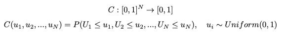
Figure 4 below shows the plot of a bivariate copula, consisting of 2 marginal distributions. The copula is defined in the [0–1]² domain (x, y-axis) and outputs values in [0–1] (z-axis):

A popular choice for C is the Gaussian Copula — the copula of Figure 4 is also Gaussian.
How we construct Copulas
We won’t delve into much detail here, but let’s give a brief overview.
Initially, we have a random vector — a collection of random variables. In our case, each random variable z_i represents the observation of a time series i at a time step t:

Then, we make our variables uniformly distributed using the probability integral transform: The CDF output of any continuous random variable is uniformly distributed,F(z)=U :

And finally, we apply our Gaussian Copula:

where Φ^-1 is the inverse standard gaussian CDF N∼(0,1), and φ (lowercase letter) is a gaussian distribution parameterized with μ and Σ . Note that Φ^-1[F(z)] = x, where x~(-Inf, Inf) because we use the standard inverse CDF.
So, what happens here?
We can take any continuous random variable, marginalize it as uniform, and then transform it into a gaussian. The chain of operations is the following:

There are 2 transformations here:
F(z) = U, known as probability integral transform. Simply put, this transformation converts any continuous random variable to uniform.Φ^-1(U)=x, known as inverse sampling. Simply put, this transformation converts any uniform random variable to the distribution of our choice — hereΦis gaussian, soxalso becomes a gaussian random variable.
In our case, z are the past observations of a time series in our dataset. Because our model makes no assumptions about how the past observations are distributed, we use the empirical CDF — a special function that calculates the CDF of any distribution non-parametrically (empirically).
In other words, at the F(z) = U transformation, F is the empirical CDF and not the actual gaussian CDF of the variable z . The authors use m=100 past observations throughout their experiments to calculate the empirical CDF.
Recap of Copulas
To sum up, the Gaussian copula is a multivariate function that uses
μandΣto directly paremeterize the correlation of two or more random variables.
But how does a Gaussian copula differ from a Gaussian multivariate probability distribution(PDF)? Besides, a Gaussian Copula is just a multivariate CDF.
The Gaussian Copula can use any random variable as a marginal, not just a Gaussian.
The original distribution of the data does not matter — using the probability integral transform and the empirical CDF, we can transform the original data to gaussian, no matter how they are distributed.
Gaussian Copulas in Deep GPVAR
Now that we have seen how copulas work, it’s time to see how Deep GPVAR uses them.
Let’s go back to Figure 3. Using the LSTM, we have computed the μ and Σ parameters. What we do is the following:
Step 1: Transform our observations to Gaussian
Using the copula function, we transform our observed time-series datapoints z to gaussian x using the copula function. The transformation is expressed as:

where f(z_i,t) is actually the marginal transformation Φ^-1(F(z_i)) of the time-series i.
In practice, our model makes no assumptions about how our past observations z are distributed. Therefore, no matter how the original observations are distributed, our model can effectively learn their behavior, including their correlation, thanks to Gaussian Copulas' power.
Step 2: Use the computed parameters for the Gaussian.
I mentioned that we should transform our observations to Gaussian, but what are the parameters of the Gaussian? In other words, when I said that f(z_i) = Φ^-1(F(z_i)), what are the parameters of Φ ?
The answer is the μ and Σ parameters — these are calculated from the dense layers and the LSTM shown in Figure 3.
Step 3: Calculate the loss and update our network parameters
To recap, we transformed our observations to Gaussian and we assume those observations are parameterized by a low-rank normal Gaussian. Thus, we have:

where f1(z1) is the transformed observed prediction for the first time series, f2(z2) refers to the second one and f_n(z_n) refers to the N-th time series of our dataset.
Finally, we train our model by maximizing the multivariate gaussian log-likelihood function. The paper uses the convention of minimizing the loss function — the gaussian log-likelihood preceded with a minus:

Using the gaussian log-likelihood loss, Deep GPVAR updates its LSTM and the shared dense layer weights displayed in Figure 3.
Also, notice:
The
zis not a single observation, but the vector of observations from allNtime-series at timet. The summation loops untilT, the maximum lookup window — upon which the gaussian log-likelihood is evaluated.And since z is a vector of observations, the gaussian log-likelihood is actually multivariate. In contrast, DeepAR uses a univariate gaussian likelihood.
Deep GPVAR Variants
From the current paper, Amazon created 2 models, Deep GPVAR (which we describe in this article) and DeepVAR.
DeepVAR is similar to Deep GPVAR. The difference is that DeepVAR uses a global multivariate LSTM that receives and predicts all time series at once. On the other hand, Deep GPVAR unrolls the LSTM on each time series separately.
In their experiments, the authors refer to the DeepVAR as Vec-LSTM and Deep GPVAR as GP.
The Vec-LSTM and GP terms are mentioned in Table 1 of the original paper.
The Deep GPVAR and DeepVAR terms are mentioned in Amazon’s Forecasting library Gluon TS.
This article describes the Deep GPVAR variant, which is better on average and has fewer parameters than DeepVAR. Feel free to read the original paper and learn more about the experimental process.