Influential Time-Series Forecasting Papers of 2023-2024: Part 2

The 2nd part of innovations in time-series forecasting

Feb 10, 2025

I hope your 2025 is off to a great start! This is Part 2 of my roundup of the most notable time-series forecasting papers from 2023-2024.

If you missed Part 1, check it out here. In this second part, I’ll also discuss impactful papers that bring key innovations from other areas of machine learning into time-series forecasting.

The papers I’ll cover are:

NHITS: Neural Hierarchical Interpolation for Time Series Forecasting (AAAI-23)
iTransformer: Inverted Transformers Are Effective For Time-Series Forecasting (ICLR ‘24)
Forecasting With Hyper-trees
SpaceTime: Effectively Modeling Time Series with Simple Discrete State Spaces (ICLR ‘23)
Mamba4Cast: Efficient Zero-Shot Time Series Forecasting with State Space Models (NeurIPS ‘24 Workshop)

Let’s get started:

Horizon AI Forecast is a reader-supported newsletter, featuring occasional bonus posts for supporters. Your support through a paid subscription would be greatly appreciated.

Also, check the AI Projects folder for some cool hands-on projects!

NHITS: Neural Hierarchical Interpolation for Time Series Forecasting (AAAI-23)

Released 2 years ago, NHITS is a battle-tested Deep Learning model — and an upgrade from N-BEATS.

I previously discussed NHITS in an earlier article, with an additional in-depth tutorial here.

NHITS: A Complete Tutorial for Deep Learning Time-Series Forecasting

Nikos Kafritsas

October 18, 2024

Read full story

NHITS is a milestone model — since it merges Deep Learning with signal processing theory. More specifically, NHITS is:

Lightweight and Efficient: Uses signal theory to enhance performance with fewer parameters, eliminating the need for many hidden layers.
Versatile: Handles past observations, future inputs, and static variables, suitable for energy demand, retail, and financial markets.
Advanced Signal Sampling: Captures complex frequency patterns using multi-rate sampling, critical for financial forecasting.
Probabilistic Forecasting: Supports quantile regression or probabilistic linear heads.
Intermittent data: Handles sparse data very well if you use e.g. a Poisson Loss distribution.

The 2 most important contributions of NHITS are:

Multi-rate sampling: Each block in the model applies a pooling strategy with a varying kernel — mimicking a sampling process per block.
Hierarchical Interpolation: Each stack in the model forecasts at a different frequency and later interpolates the predictions to form the full prediction length. Hence, each stack focuses on a specific frequency.

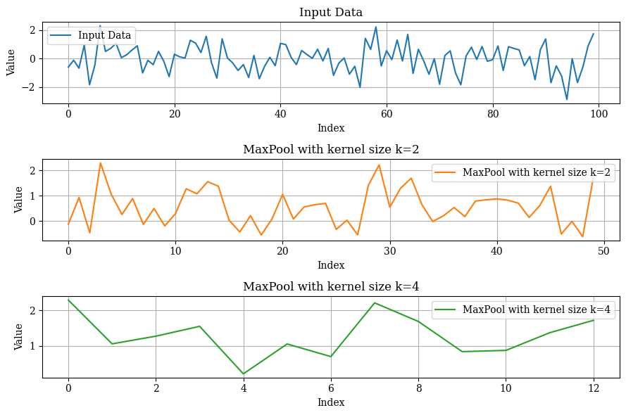
**Figure 1:** *The effect of applying MaxPooling to the input signal with different k kernel sizes (Image by author)*

**Figure 2:** Hierarchical Interpolation. Each stack has a different expressiveness ratio (1/r), with r > 0. Given horizon H, each stack predicts (1/r)×H data points. The top stack (stack 1) has a lower ratio, focusing on lower frequencies and heavier interpolation. As the stack level increases, the ratio grows, shifting the focus to higher frequencies (Source [1])

In my AI Projects folder companion notebook (Project 2) I demonstrate how to reproduce the above graphs.

The architecture of NHITS is shown in Figure 3:

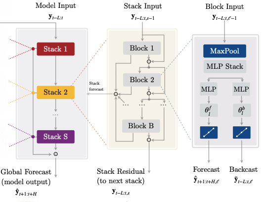
**Figure 3:** *Computations flow from right to left – basic block (right), stack of blocks (middle), stack of stacks (left) (Source [1])*

NHITS is a modular model, consisting of blocks and stacks. This makes the model more sparse and lightweight, with each block specializing in a different frequency.

If you’re working on a forecasting project, NHITS is worth trying—it’s versatile and even trainable on a CPU. In Nixtla’s mega-study (discussed here), NHITS was among the top models.

iTransformer: Inverted Transformers Are Effective For Time-Series Forecasting (ICLR ‘24)

As discussed in Part 1, early 2023 saw Transformer-based forecasting models exploring various embedding strategies.

iTransformer attempts multivariate forecasting by embedding across the time dimension rather than the feature dimension. I’ve written an in-depth article about iTransformer, with a long-term forecasting tutorial here.

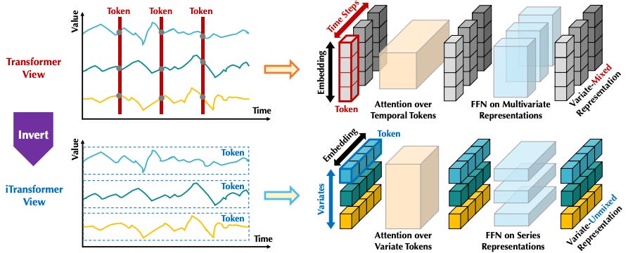
**Figure 4:** *Core operations in iTransformer’s architecture. The embedding operation tokenizes across time(variate tokens) not feature dimension. (Source [2])*

Traditional Transformer-based models embed information across the feature dimension. This is problematic, leading to the following issues:

Lagged Information: In practice, dependencies can be lagged, such as yi depending on xi-1 rather than xi. Time-based embeddings may overlook these lags.
Limited Receptive Field: Unlike NLP, where words are discrete, time-series data is continuous. Tokenizing by timepoints restricts the model’s receptive field, failing to capture long-term correlations.

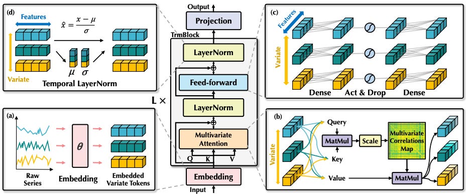
iTranformer solves these by “inverting” the embedding scheme — tokenizing each time series independently to create variate tokens. Self-attention is then applied across these tokens, capturing interdependencies:

**Figure 5:** *Comparing vanilla Transformer(top) and iTransformer(bottom) (Source [2])*

iTransformer also offers key advantages:

No Positional Embeddings: Temporal order is captured by MLPs after attention.
Faster Self-Attention: Attention applies only across variate tokens.
Better Interpretability: Self-attention weights reveal multivariate correlations, which can be visualized for insights.

Also, iTransformer excels in long-term forecasting. A tutorial benchmarking iTransformer and TSMixer is available here:

**Figure 6:** iTransformer predictions on the ETTm2 dataset with horizon = 96, compared to TSMixer and other models *(Image by author)*

So, which model to use?

There’s no one-size-fits-all model for time-series forecasting. In part 1 we discussed CARD and TSMixer. To recap:

NHITS: Best for datasets with exogenous and future-known variables, assuming no explicit dependencies.
TSMixer-Ext: Ideal when external covariates exist but have more complex interdependencies (e.g., retail cases like M5).
iTransformer or CARD: Best for large datasets requiring cross-variate modeling. CARD also supports static variables.

Forecasting With Hyper-trees

The built-in ensembling nature of Gradient Boosted Trees makes them ideal for time series forecasting.

However, they have a key limitation—trend extrapolation. Trees cannot predict values beyond their training range. This can be mitigated with detrending techniques (e.g. using an extra linear model or performing decomposition). LightGBM offers a linear_tree parameter, which fits linear models at the leaves. Each method has trade-offs.

A recent study addressed this challenge by introducing Hyper-Trees, a hybrid approach based on Hyper-Networks:

A Hyper-Tree is a modular GBDT-based model that parameterizes a target model—such as ARIMA, ETS, or an MLP—specifically for time series forecasting.

Advantages of Hyper-Trees:

Tailored for Time Series: They can natively extrapolate trends without extra feature engineering.
Fusion: They integrate statistical models (effective for local setups) or ANNs (ideal for global setups leveraging cross-variate information).
Versatile: Can be used for forecasting or decomposition (e.g., like STL).
Interpretability: Using SHAP values for parameter estimates enhances the interpretability of time series models.
Operationally Robust: They Inherit GBDT advantages, including handling missing data and exogenous variables.
Minimal Feature Engineering: No need to manually add lagged target variables as extra features

The top-level view of Hyper-Trees is illustrated below:

**Figure 7:** *Illustration of Hyper-Trees (Source [3])*

Essentially, a Hyper-Tree parameterizes a target model (it could be a statistical or an MLP) whose output uses a loss function to derive Gradients and Hessians that help update the GBDT next. The authors use LightGBM as the GBDT backbone - but it can be any GBDT

The authors demonstrate 3 basic functionalities of Hyper-Trees:

Seasonal Decomposition

Hyper-Trees can function as a decomposition method, similar to STL.

They achieve this by parameterizing functions that capture trend and seasonality:

where

\(\Theta_{\sigma}(x_t) = [\theta_{0,t}(x_t), \theta_{1,t}(x_t), \theta_{\text{sine},t}(x_t), \theta_{\text{cosine},t}(x_t)]\)

The Theta parameters are modeled as functions of time-derived features x_t = {month, quarter, year, time}, with time being a linearly increasing integer.

This variant is called Hyper-Tree-STL and produces results comparable to traditional STL.

**Figure 8:** *Hyper-Trees vs STL*(Source [3])

The paper describes additional capabilities and shows how to use these parameters to extract feature importances. For more information, read the original paper.

Local Time Series Model

Hyper-Trees can parameterize statistical models like AR(p) and ETS.

For example, they can learn a probabilistic distribution probabilistic distribution N(μ,σ) where an AR process parameterizes μ:

\(\mu_t = \theta_{1,t}(x_t)y_{t-1} + \theta_{2,t}(x_t)y_{t-2} + \cdots + \theta_{p,t}(x_t)y_{t-p} \\)

\(\sigma_t = \text{softplus}(\theta_{a,t}(x_t))\)

and θ’s are parameters estimated by the Hyper-Tree.

This model’s architecture is illustrated below:

**Figure 9:** *A Hyper-Tree parameterizing an AR(p) process ((Source [3])*

Notes:

The order of p in the AR model can be selected based on seasonality.
The authors experiment with additional statistical models.
Unlike traditional trees, Hyper-Trees perform gradient descent in parameter space rather than function space, meaning each tree produces a distinct parameter (this is my understanding from reading the paper)

Global Time Series Model

The authors also propose GBM-Net, a Hyper-Tree variant for global forecasting models.

This variant now parameterizes an MLP — intending to fit a global model across all time series (Figure 10)

This mimics an encoder-decoder architecture — the tree is the encoder and the MLP is the decoder.
The tree and the MLP are jointly trained.

**Figure 10:** *A Hyper-Tree parameterizing an MLP (Source [3])*

The paper includes an extensive benchmark across various models and datasets.

What I liked in this paper is the authors don't just present a new model with SOTA results—they analyze multiple scenarios, demonstrating where Hyper-Trees excel and how they should be used.

The original paper is worth reading, and the authors plan to release the code soon.

SpaceTime - Effectively Modeling Time Series with Simple Discrete State Spaces (ICLR 23)

State-space models(SSMs) represent dynamic systems with state variables and equations.

For example, the Kalman filter is an SSM. RNNs also fall under SSMs. Recently, researchers revisited SSMs as a solution to Transformers' shortcomings.

Let’s briefly review these architectures—and then explore 2 milestone time-series papers leveraging SSMs.

Preliminaries

Transformers and RNNs have distinct advantages and drawbacks. Let’s compare them using a sentence as input:

Transformers

Unbounded Context within Input: Each word in the sentence can attend directly to itself and every other word of the sentence.
Highly Parallelizable: Training is highly parallelizable due to self-attention.
Slower Inference: Autoregressive prediction is slow since attention matrices must be recomputed at each step (e.g. for generating the next word).

RNNs

Limited Context: The hidden state, which updates at each step, allows indirect access to only previous words.
Training Bottlenecks: No parallelization in training due to sequential updates, leading to vanishing/exploding gradients.
Efficient Inference: They process sequences step by step, maintaining a hidden state indefinitely - this enables efficient long-sequence processing.
Unbounded Generation: Can theoretically generate outputs indefinitely by updating the hidden state regardless of the input length.

Note: Recent Transformer advancements like key-value (KV) caching improve inference speed and reduce memory usage by avoiding redundant recomputation.

To sum-up:

**Table 1:** *Transformers vs RNNs (Source: Author)*

Why do we need SSMs?

Despite their dominance, Transformers suffer from slow inference.

Here come SSMs, and we’ll specifically discuss NN-based SSMs. The goal is to find an architecture that balances context handling, training, and inference efficiency.

The basic SSM structure is illustrated in Figure 11:

**Figure 11:** *Basic State-Space Model Diagram (Image by Author)*

The equations of an SSM are as follows:

\( x' = \mathbf{A}x + \mathbf{B}u\)

\( y = \mathbf{C}x + \mathbf{D}u\)

where:

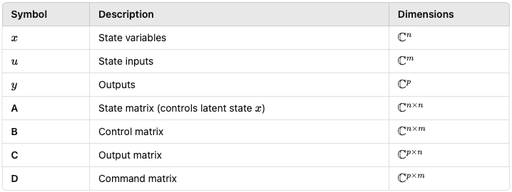
Figure 11 depicts the continuous-time view.

The idea is to use an SSM with 3 views. Continuous-time view, Convolutive, and Reccurent. Specifically:

Continuous-time view: Here, we can represent any type of continuous data(audio, time series, etc) but training and inference are slow.
Convolutive view: Convolutions enable efficient parallel training, unlike RNNs, which are sequential and slower.
Recurrent View: RNNs offer theoretically unbounded context and constant-time state updates—ideal for inference.

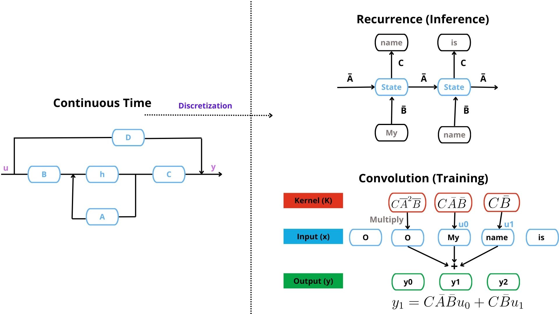
**Figure 12:** *The 3 views of a State-Space model (Image by author)*

Since input data is continuous, SSMs primarily use the continuous-time representation. But it’s analytically challenging to solve the equations in the continuous form. Plus, if the data is discrete (e.g. text), discretization is necessary.

The core strength of NN-based SSMs lies in their ability to transition from the continuous-time form to the convolutive form for training and the recurrent form for inference.

We’ll explore these in more detail in a future article. For a deeper dive into SSMs, I recommend the Annotated S4 blog (in JAX) and its PyTorch counterpart. S4 is a popular NN-based SSM model— and the predecessor of Mamba (more on this later).

Enter SpaceTime

Developed by Stanford's Hazy Research lab (led by Professor Christopher Ré), SpaceTime is an SSM model based on S4 adapted specifically for time series.

Note: The Hazy Research lab extensively studied SSMs, publishing milestone models like S4 and Mamba. They’ve also introduced Hyena, a Transformer alternative, among other significant contributions—take a look at their work!

Key advantages of SpaceTime:

Versatile: Supports both forecasting and classification.
Open-Source: The model is open-source — you can find it here.
Tailored for time series: The SSM parameterizes the matrix A — which the authors proved can represent various statistical models like ARIMA and ETS.
Built-in Time-Series Preprocessing. The C matrix is adapted to apply differencing and moving average smoothing — helping the model handle non-stationary data and noise natively.
Long-range Forecasting: Instead of standard autoregressive forecasting (which accumulates errors), SpaceTime introduces a closed-loop mechanism in its final layer. This forecasts its own future inputs, mimicking multi-step prediction.
Efficiency: Leverages convolutions for fast training and recurrence for dynamic forecasting. Additionally, inference is further optimized using convolutions for specific operations.

Like other SSMs that optimize state matrix A, SpaceTime also introduces new parameterizations:

where a’s are learnable parameters.

By configuring the rest of the variables as follows:

The authors prove that the following SSM’s equations:

Can represent an AR(p) process:

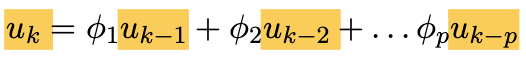
as well as other temporal functions.

The top-level view of SpaceTime is illustrated in Figure 13:

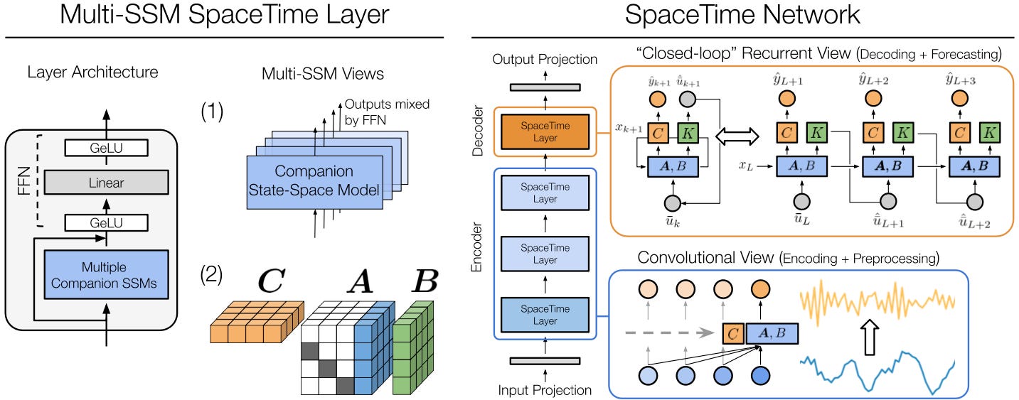
**Figure 13:** *The architecture of SpaceTime and its core layers (Source [4])*

The authors made additional optimizations, including:

An efficient FFT-based algorithm to accelerate convolution.
Computing multiple SSMs to enhance the model's expressiveness.
Instead of using S4’s diagonal and low-rank format, they use shift and low-rank in matrix A

For more details, check the original paper—it includes insightful proofs explaining the model's design choices and useful benchmarks.

Mamba4Cast: Efficient Zero-Shot Time Series Forecasting with State Space Models (NeurIPS ‘24 Spotlight Workshop)

The evolution of NN-based State Space Models (SSMs) from S4 to S5 follows a common theme—combining convolutions with recurrence.

After S5, the family split into two branches: Hyena (CNN-focused) and Mamba (recurrence-focused), leading to Mamba-2.

Mamba (also called S6) introduced selective state spaces, which apply a filtering function to the B and C matrices, guiding the model on what parts of inputs and outputs to focus on.

Think of selective state spaces as a middle ground between recurrence (which only accesses the previous hidden state) and self-attention (which attends to all inputs simultaneously).

If you're interested in Mamba, drop a comment—we’ll explore it in a future article.

Quick Reference:
S4: Structured State-Space sequence model
S5: Structured State-Space sequence model with scan
S6(Mamba): Structured State-Space Selective sequence model with scan

Mamba was initially built as a language model, but it has since found applications in image processing (Vision Mamba) and video (VideoMamba). We can also replace the Mamba block with a Transformer block in some architectures.

One emerging application of Mamba is time-series forecasting. Several Mamba variants have been developed for this, including Mamba4Cast.

Enter Mamba4Cast

Mamba4Cast, built on Mamba-2, is designed for time-series forecasting.

Key features:

It’s based on Mamba-2, a recurrent architecture demonstrating faster inference than Mamba.
It’s an open-source model.
It contains 27M parameters (relatively small for a foundation model).
It’s pretrained on synthetic data and works as a foundation model like TimesFM and MOIRAI.

Figure 14 shows the model’s architecture:

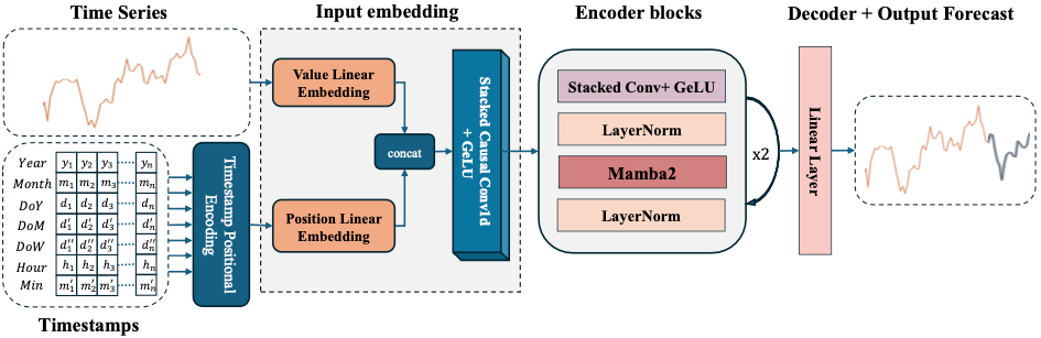
**Figure 14:** *Mamba4Cast top-level view (Source [5])*

Here are the basic layers/components of Mamba4Cast:

Pre-processing: Scales input series with a Min-Max Scaler and extracts time features for positional embeddings.
Embedding: Uses dilated convolutions to embed scaled values and temporal information, ensuring a large receptive field.
Encoder: Composed of Mamba2 blocks with LayerNorm to stabilize learning, followed by a dilated convolution layer.
Decoder: A linear projection layer transforms embedded tokens into point forecasts.

Since Mamba4Cast is a foundation model, it’s benchmarked against other foundation models and SOTA forecasting models. Check out the original paper for details.

Unlike NLP, Transformers aren’t a silver bullet in time-series forecasting. Deep State-Space Models like Mamba offer a modern, competitive alternative—worth exploring if you're looking for a fresh approach.

Thank you for reading!

Horizon AI Forecast is a reader-supported newsletter, featuring occasional bonus posts for supporters. Your support through a paid subscription would be greatly appreciated.