TimesFM: Google's Foundation Model For Time-Series Forecasting
A New Age for Time Series
Welcome to the 3rd edition!
In August 2023, the time-series community was disrupted by the release of TimeGPT, Nixtla's first foundation model for time series forecasting.
We covered this here:
Following TimeGPT, multiple foundation forecasting models were released, but there was one that stood out. Recently, Google unveiled TimesFM, a groundbreaking time-series model with phenomenal results.
In this article, we discuss:
The challenges of foundation models in time series compared to NLP.
How TimesFM overcomes these challenges.
How TimesFM works and why it’s a powerful model.
TimesFM benchmark results.
Prospects for the future of foundation models in time-series forecasting
Let's get started.
Horizon AI Forecast is a reader-supported newsletter, featuring occasional bonus posts for supporters. Your support through a paid subscription would be greatly appreciated.
Why Foundation Models are Challenging for Time Series?
The concept of a promising foundation model in NLP was already evident with the release of GPT-2 in Language Models are Unsupervised Multitask Learners.
But in time series, building a foundation model is not straightforward. There are several challenges:
Dataset Scarcity: In NLP, finding text data is easy. We can scrape large amounts of unstructured data (from the Web) or high-quality data (books, articles, etc.). However, public time-series datasets are not readily available.
Unpredictable Format: Language models are based on well-defined grammars and vocabularies. Time-series data may belong to domains with different characteristics—e.g., highly sparse sales or volatile financial data.
Different Granularities: Each time series model works for a specific granularity—e.g., hourly, weekly, monthly, etc. How can a time-series foundation model work well for every granularity?
Variable Contexts and Horizons: NLP models have a predefined max context length and are optimized to predict the next word. A universal time-series model should work for variable context lengths and horizons.
Enter TimesFM
TimesFM is a foundation Time-Series Forecasting model, created by Google Research.
More specifically, TimesFM:
Has 200M parameters.
Was trained on 100 billion real-world time-points.
Allows extra covariates as features.
Leverages Causal Self-Attention and Residual Blocks.
Outperforms other SOTA models in zero-shot forecasting.
Next, let’s examine how TimesFM overcomes the challenges of building a foundation time-series model.
Note: Find a tutorial of TimesFM the AI Projects folder — this folder is constantly updated with fresh tutorials on the latest time-series models!
A) Finding Vast Amounts of Data
Public time-series datasets are scarce.
Standard benchmarks like the Monash repository (which contains popular datasets, e.g. Tourism, Electricity) can only get you so far.
An ideal dataset for a universal time-series model should have:
A large volume of data (in the order of millions)
Diverse data - representing multiple domains
Every time granularity (daily, weekly, etc)
The TimesFM authors managed to leverage 3 additional resources from public time-series data:
Google Trends: The authors repurposed Google Trends search interests over time as time-sequences.
Wiki Pageviews: These capture the hourly views of all Wikimedia pages.
Synthetic Data: The authors used ARMA processes to create a corpus of time series that featured mixed seasonalities, frequencies, and trends.
The result was a dataset of 100 billion datapoints.
However, 100B datapoints pale in comparison to the 1T tokens of LLaMa! Still, it’s a good start toward creating large-scale time-series datasets.
B) Variable Contexts and Horizons
So far, we have a large and diverse dataset containing datapoints from multiple domains and time granularities.
A large Transformer could learn universal temporal patterns. But what assumptions should we make about the context length and the horizon?
Research on Horizon Length (Prediction Length)
LLMs are optimized to predict the next word (autoregressive).
Regarding time-series models, 2 issues arise:
Research has shown [Zhou et al.] [Makridakis et al.] that directly predicting the full horizon, instead of using a multi-step autoregressive approach, works better in long-term forecasting.
However, in our case (zero-shot forecasting) this is not possible when the horizon length is not known apriori. A universal model should be able to predict any horizon length.
TimesFM finds a middle ground by leveraging patching, a technique popularized by another successful model, PatchTST.
How Patching Works
TimesFM does not predict one data point at a time, nor does it predict the full horizon length. Instead, it breaks down both the context and horizon length into patches.
Assume we have:
a context-length of size L,
and patches of size p,
then we break the input into N = L/p patches. These are called input patches.
We also have output patches of size h(horizon).
By allowing
output_patch_size>input_patch_size, authors found that TimesFM can learn to predict a horizon of any length faster and more accurately.
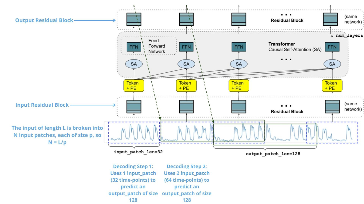
Figure 1 shows the TimesFM architecture during training:

First, choose a value p for the input_patch_size, and a value of h for the output_patch_size. The model then breaks the input into N = L/p input patches.
During the first training decoding step:
The first patch is processed by an Input Residual Block.
The result is added to a positional encoding vector.
The output of step 2 is fed to a stacked Transformer. There, causal self-attention is applied so that each output token can only attend to the input tokens before it.
Similarly, the output of step 3 is passed to an Output Residual Block - thus creating the output patch, which is the predictive horizon. This patch is compared with the actual data to calculate the loss.
In the next decoding step, the model will process the first two input patches, and output the second output patch.
Note: In practice, all patches for a given input are created in one training mini-batch.
Example of Figure 1
During training, assuming
input_patch_size=32andoutput_patch_size=128:The model is simultaneously trained to use the first 32 time-points to forecast the next 128 time-steps, the first 64 time-points to forecast time-steps 65 to 192, the first 96 time-points to forecast time-steps 97 to 224, and so on.During inference, suppose the model is given a new time series of length 256 and tasked with forecasting the next 256 time-steps into the future, with
input_patch_sizeandoutput_patch_sizeas defined in Figure 1:
The model will first generate 128 future predictions for time-steps 257 to 384, then condition on the initial 256 length input plus the generated output to generate another 128 predictions — that’s time-steps 385 to 512.
In other words:
TimesFM is trained in decoder-only mode, similar to GPT models. The difference is in treating each token as a patch of time-points. Patching significantly improves inference speed and avoids constraining the model to a specific prediction length/horizon.
And there you have it! We have outlined the architecture of TimesFM.
Note: In addition to the patch, a masking vector is supplied - randomly masking a portion of the patch. This is done to prevent the model from only learning to predict for context_lengths that are multiples of the input patch length.
Evaluation Benchmarks
Finally, the authors evaluated TimesFM against other SOTA forecasting models (statistical, tree-based, deep-learning).
Also, the authors benchmarked llmtime, another successful TS foundation model that uses GPT-3 and LLaMa-2 with specific modifications tailored for time-series forecasting.
The benchmark parameters are as follows:
Scaled MAE is used — each model’s MAE is scaled by the MAE of a naive baseline model since datasets have different scales.
All models are evaluated on a hold-out dataset.
TimesFM is zero-shot here — it wasn’t pretrained on the held-out data.
Conversely, all the other models were explicitly trained and fine-tuned on the held-out data.
The hold-out data consists of time series belonging to 3 datasets: The Monash Archive, the Darts data benchmark, and the Informer benchmark. The same datasets were used to evaluate llmtime.
The evaluation results are shown below:


Notes regarding the results:
TimesFM is the clear winner here
TimesFM is among the top-3 models in every benchmark — surpassing llmtime as well.
Remember, TimesFM does zero-shot inference here — meaning that TimesFM had never seen that data during training! In contrast, the other models were individually trained on the time series of the hold-out set.
Also, all 3 benchmarks contain datasets that cover various domains, sizes, granularities, and horizon lengths. Achieving such competitive results on diverse and unseen data is an impressive feat — a trend also observed in the TimeGPT benchmark.
The impact of fine-tuning
The TimesFM paper lacks details on the effect of fine-tuning.
Zero-shot inference is an excellent way to evaluate a foundation model. But how the results would have improved if TimesFM had been fine-tuned on a portion of the evaluation data?
Besides, fine-tuning is a standard practice in NLP. Interestingly, neither TimesGPT shares any fine-tuning training details, but its API allows fine-tuning on your own dataset.
Scaling Laws
TimesFM is essentially a large pretrained decoder-only Transformer model, so it makes sense to evaluate its performance in terms of the model size. To recap:
Scaling laws are empirical rules that describe the relationship between an LM’s parameter size, tokens(dataset size), training time, and performance.
Scaling laws were first introduced by [Kaplan et al], but later refined by [Hoffman et al], also known as the Chinchilla paper.
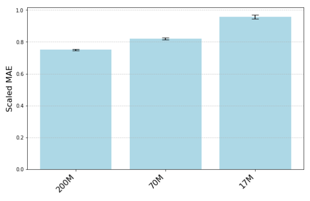
Naturally, TimesFM authors performed a preliminary scaling study where they trained 3 TimesFM models of sizes 17M, 70M, and 200M parameters, using the same pretraining dataset and till a similar number of iterations.
The results are shown in Figure 4:

Clearly, the model scales with more parameters, proving that scaling laws also apply in Transformer forecasting models (as shown in [Kunz et al.]).
Moreover, the authors examined the effect of the dataset size on the model performance. They compared the performance by training only on smaller datasets (M4, Electricity, Traffic, and Weather) vs larger datasets (Google Trends, etc.) & synthetic. The results are shown in Figure 5:

It would have been more interesting if the other relationships were also included in the study with more details — specifically the performance vs dataset size and the performance vs training time relationships.
Ablation study
Finally, the authors conduct an ablation study to measure the impact of their architectural choices.
They mostly focus on the relationships between the performance of TimesFM and the sizes of the input and output patches.
Remember, the choice of breaking the input into patches and allowing the output patches to be larger is the key design choice of TimesFM. If we didn’t have input patches (e.g., the model consumed the full input in a single step), TimesFM would essentially function as an encoder-decoder model, not decoder-only.
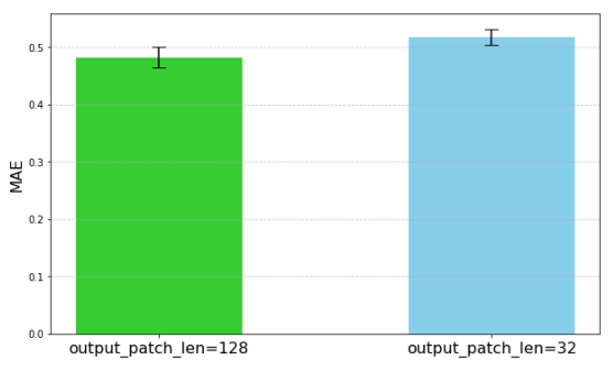
Therefore, the authors measured how the performance and the size of input/output patches are related. The analysis is shown in Figure 6 and Figure 7:


Both figures justify choosing a smaller input patch (though not very small) and a larger output patch—effectively making TimesFM a decoder-only model.
Closing Remarks
TimesFM is a phenomenal TS model by Google — and a crucial addition to the category of TS foundation models.
Currently, the model is in private beta, but Google plans to make it available on Google Cloud Vertex AI. But neither the model nor the training dataset have been made available (Google is still contemplating whether to open-source the model).
Fortunately, the TimesFM paper is much more informative than Nixtla’s TimesGPT paper — providing numerous insights into what a foundation forecasting model entails.
Still, research on TS foundation models has a long way to go, considering the absence of a large public time-series dataset. For context, when T5 was released in 2019, the C4 dataset (750GB of cleaned text data derived from CommonCrawl) was already available.
In my opinion, there’s great potential for TS foundation models in the future!
Thank you for reading!
Horizon AI Forecast is a reader-supported newsletter, featuring occasional bonus posts for supporters. Your support through a paid subscription would be greatly appreciated.


