
Temporal Fusion Transformer: Time Series Forecasting with Interpretability
Generate accurate and interpretable forecasts

Temporal Fusion Transformer (TFT) [1] is a proven Transformer-based forecasting model.
TFT recently gained attention again during the VN1 [2] forecasting competition. Antoine Schwartz, a participant, used TFT to achieve 4th place overall — and 1st as a non-ensemble model.
Interestingly, if ensembling had been applied, Antoine could have scored even higher, possibly securing 1st place overall.
Figure 1 below shows the results of the top 22 participants:

The VN1 is an interesting competition, with many great insights. For example, Evandro Cardonzo da Silva secured 12th place with a Naive model! Yes, it seems surprising at first— but this highlights the importance of establishing strong baselines!
In this article, we focus on the Temporal Fusion Transformer. We’ll explore its architecture, how it works, and why it’s a strong model.
Moreover, a key advantage of TFT is its native interpretability features. It includes a custom self-attention mechanism that provides valuable insights:
Seasonality Analysis
Feature Importances
Rare Event Robustness
I’ll also explain these interpretability mechanisms in detail. Let’s get started!
✅ Find the hands-on project for TFT in the AI Projects folder. I’ll soon add a volatility forecasting case using TFT — so stay tuned!
You can also support my work by subscribing to AI Horizon Forecast:
Enter Temporal Fusion Transformer (TFT)
The Temporal Fusion Transformer (TFT) is a Transformer-based model that leverages self-attention to capture complex temporal patterns across multiple time sequences.
Some key features of TFT are:
Multiple time series: TFT can train on thousands of univariate or multivariate time series.
Multi-Horizon Forecasting: The model generates multi-step predictions for one or more target variables — including prediction intervals.
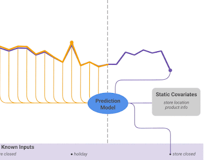
Heterogeneous features: TFT supports many types of features, including past observed inputs, future known inputs, and static exogenous variables (Figure 2).
Interpretable predictions: Predictions can be interpreted in terms of variable importance and seasonality.
Probabilistic Forecasting: The model supports prediction intervals via quantile forecasts. You can further enhance TFT by conformalizing the prediction intervals.

yhat represents the qth quantile prediction for the τ-step-ahead forecast at time t, where q ∈ [0..1]. (Image by author)
Figure 3 illustrates the top-level architecture of Temporal Fusion Transformer:

For a given timestep t, a lookback window k, and a τmax step ahead window, where t⋹ [t-k..t+τmax], the model takes as input: i) Observed past inputs x in the time period [t-k..t], future known inputs x in the time period [t+1..t+τmax] and a set of static variables s (if it exists).
Next, we will break down each component step-by-step and explain how they interact.
Temporal Fusion Transformer Components
Gated Residual Network (GRN)
Figure 4 displays the Gated Residual Network (GRN) — a basic block of TFT:

Key points:
As shown in Figure 3, GRN appears in multiple layers. It can function as a standalone component or as part of the Variable Selection Network.
It has 2 dense layers and two types of activation functions - called ELU (Exponential Linear Unit) and GLU (Gated Linear Units). GLU, originally introduced in Gated Convolutional Networks [4], helps select the most important features for predicting the next word.
The final output passes through standard Layer Normalization. The GRN also contains a residual connection - helping the flow of the gradients.
Depending on its position in TFT, the GRN can leverage static variables.
Variable Selection Network (VSN)
As the name suggests, the VSN acts as a feature selection mechanism (Figure 3). Recall:
Not all time series are complex. The model must distinguish meaningful features from noisy ones. Since TFT handles 3 types of inputs, it uses 3 types of VSN (represented by different colors in Figures 3 and 5).

Naturally, the VSN utilizes GRN for its filtering capabilities. This is how it works:
At time
tthe flattened vector of all past inputs (calledΞ_t) of the corresponding lookback period is fed through a GRN unit (in blue) and then a softmax function, producing a normalized vector of weightsu.Moreover, each feature passes through its own GRN, which leads to the creation of a processed vector called
ξ_t, one for every variable.The final output is a linear combination of ξ_t and u.
Note that each variable has its own GRN, but the same GRN is applied across all time steps during a single lookback period.
The VSN for static variables does not consider the context vector
c -given that VSN in that case has already access to static information.
LSTM Encoder Decoder Layer
The LSTM Encoder-Decoder Layer, widely used in NLP, is shown in Figure 3. This component serves 2 purposes:
Context-Aware Embeddings: After passing through the VSN, inputs are encoded and weighted. Since the data is time-series, the model must capture sequential dependencies. The LSTM Encoder-Decoder produces context-aware embeddings (ϕ), similar to the positional encoding in Transformers (e.g., sine and cosine signals).
Why use an LSTM Encoder-Decoder instead of positional encoding?
TFT processes various input types. Known past inputs are fed into the encoder, while known future inputs go into the decoder. This suits TFT’s ability to process heterogeneous inputs in different ways.
Conditioning on Static Information: Static context vectors c cannot simply merge with the LSTM's embeddings – this would mix temporal and static information. Instead:
The initial hidden state (h_0) and cell state (c_0) of the LSTM are initialized using c_h and c_c, produced by the static covariate encoder.
As a consequence, the final context-aware embeddings
φwill be properly conditioned on the exogenous information, without altering the temporal dynamics.
Interpretable Multi-Head Attention
Finally, we apply the self-attention mechanism — helping the model learn long-range dependencies across time steps.
Transformer-based architectures leverage Attention to capture complex dependencies in input data. Contrary to traditional self-attention, TFT introduces a novel, interpretable Multi-Head Attention mechanism that enables feature interpretability.
In the original architecture, each "head" (Query/Key/Value weight matrices) projects the input into separate representation subspaces. The drawback of this approach is that the weight matrices have no common ground and thus cannot be interpreted.
TFT’s multi-head attention uses a different grouping such that the different heads share the same Values weight matrix Wv — making its attention scores now interpretable.
Quantile Regression
While point forecasts are useful, prediction intervals are crucial for decision-making.
Standard linear regression uses ordinary least squares (OLS) to estimate the conditional mean of the target variable based on feature values. OLS assumes constant variance in residuals, which often doesn't hold.
Quantile regression extends simple linear regression by estimating the conditional median — and other percentiles — of the target variable.
Figure 6 illustrates how percentiles(as prediction intervals) appear in a regression problem:

Given y (actual value), yhat (prediction), and q (quantile value between 0 and 1), the quantile loss is defined as:

As the quantile q increases, the loss penalizes underestimations more and overestimations less. Check the example below, also illustrated in Figure 7:
Think about it:
A prediction at q=0.9 means we are 90% confident the observed value lies below the prediction. For example:


However, if at q=0.9 we predict less than the true value y>y’, then something is wrong with the model. In that case:

leading to a dramatically higher loss.
Temporal Fusion Transformer is trained by minimizing the quantile loss summed across q ⋹ [0.1, 0.5, 0.9]. TFT can also be made probabilistic by incorporating distribution-based losses, such as in DeepAR, where the model learns distribution parameters (e.g. normal) and generates forecasts by sampling.
Interpretable Forecasting
Accurate forecasting is important, but so is explainability.
Deep Learning models are often criticized as black boxes. While methods like LIME and SHAP offer partial explainability, they are not effective for time-series data. Additionally, they act as external, post-hoc tools, independent of the models they explain.
Temporal Fusion Transformer provides 3 types of interpretability:
Seasonality-wise: TFT’s Interpretable Multi-Head Attention mechanism measures the importance of past time steps.
Feature-wise: TFT’s Variable Selection Network (VSN) calculates the significance of each feature.
Rare Events Analysis: TFT allows us to analyze time-series behavior during rare events.
✅ Note: The plots below are from Project 3 of the AI Projects folder — which uses TFT for energy-demand forecasting
Seasonality-wise Interpretability
TFT’s attention weight scores can highlight temporal patterns across past time steps.
Let’s plot the attention scores we calculated in the TFT tutorial of the AI Projects folder - denoted by gray lines in Figure 8:

The attention scores reveal how impactful those time steps are when the model outputs its prediction. The small peaks reflect the daily seasonality, while the higher peak towards the end probably implies the weekly seasonality.
By averaging attention scores across all time steps and series, we observe the symmetrical shape shown in Figure 9 (TFT Paper - Electricity dataset).

Question: Why is this useful? Can’t we estimate seasonality with ACF plots or time signal decomposition etc.?
Answer: Yes, but TFT’s attention weights offer additional insights:
They confirm the model captures clear seasonal dynamics.
They can reveal hidden patterns since attention considers all past inputs across covariates and time series.
Unlike autocorrelation plots, which focus on specific sequences, attention weights assess the impact of time steps across all inputs.
Feature-wise Interpretability
The Variable Selection Network component of TFT can easily estimate the feature importances:

In Figure 10, we notice the following:
The
hourandday_of_weekhave strong scores, both as past observations and future covariates. The benchmark in the original paper shares the same conclusion.The
power_usageis obviously the most impactful observed covariate.The
consumer_idis not very significant here because we use only 5 consumers (time series). In the TFT paper, where the authors use all 370 time series, this variable is more significant.
Note: In our project, we call a consumer a unique time series. Thus, the
consumer_idis the time series id.
Rare Event Analysis
Time series are notorious for being susceptible to sudden changes in their properties during rare events (also called shocks).
Even worse, those events are very elusive. Imagine if your target variable becomes volatile for a brief period because a covariate silently changes behavior:
Is this some random noise or a hidden persistent pattern that escapes our model?
With TFT, we can analyze the robustness of each feature across their range of values. Unfortunately, the current dataset does not exhibit volatility or rare events — those are more likely to be found in financial, sales data, and so on. Still, we show how to calculate them below.
Some features do have not all their values present in the validation dataset, so we only show the hour and consumer_id:

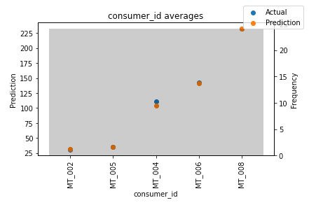
In both Figures above, the results are encouraging. In Figure 12, the time series MT_004 slightly underperforms compared to others. We could verify this if we normalize the P50 loss of every consumer with their average power usage (check Project 3 here)
The gray bars display each variable’s distribution. A good practice is to identify low-frequency values and examine model performance in those areas. This helps detect whether the model effectively captures rare event behavior.
In general, you can use this TFT feature to probe your model for weaknesses and proceed to further investigation.
Closing Remarks
Temporal Fusion Transformer marks a significant milestone for the time-series community.
Many practitioners hesitate to adopt deep learning for forecasting due to high computational costs.
However, with increased access to GPUs, these models can now be easily tuned and—under the right configurations—can outperform Gradient Boosted Trees.
TFT's native interpretability and its ability to handle diverse input features make it an excellent choice for domains like demand planning, retail, and financial markets, where a variety of features are utilized.
References
[1] Bryan Lim et al., Temporal Fusion Transformers for Interpretable Multi-horizon Time Series Forecasting, September 2020
[2] Vandeput, Nicolas. “VN1 Forecasting - Accuracy Challenge Phase 2.” DataSource.ai, 3 Oct. 2024, https://www.datasource.ai/en/home/data-science-competitions-for-startups/phase-2-vn1-forecasting-accuracy-challenge/description
[3] Vandeput, Nicolas Linkedin Post
[4] Y. Dauphin et al., Language modeling with gated convolutional networks, ICML, 2017
Thank you for reading!
Horizon AI Forecast is a reader-supported newsletter, featuring occasional bonus posts for supporters. Your support through a paid subscription would be greatly appreciated.