TIME-MOE: Billion-Scale Time Series Foundation Model with Mixture-of-Experts

And open-source as well!

A top-level view of Time-MOE (Image Source)

The Mixture-of-Experts (MOE) architecture has surged in popularity with the rise of large language models (LLMs).

As time-series models adopt cutting-edge techniques, Mixture-of-Experts has naturally found its place in the time-series foundation space.

This article discusses Time-MOE, a time-series foundation model that uses MOE to improve forecasting accuracy while reducing computational costs. Key contributions include:

1. Time-300B Dataset: The largest open time-series dataset, with 300 billion time points across 9 domains, and a scalable data-cleaning pipeline.

2. Scaling Laws for Time Series: Insights into how scaling laws affect large time-series models.

3. Time-MOE architecture: A family of open-source time-series models leveraging MOE to enhance performance.

Let’s get started

✅ Find the hands-on project for Time-MOE in the AI Projects folder (Project 11), along with other cool projects!

Enter Time-MOE

Time-MOE is a 2.4B parameter open-source time-series foundation model using Mixture-of-Experts (MOE) for zero-shot forecasting

Key features of Time-MOE:

1. Flexible Context & Forecasting Lengths: Handles context lengths up to 4096 timepoints and any forecasting horizon.

2. Sparse Inference: MOE activates only a subset of parameters during prediction.

3. Lower Complexity: The largest variant, Time-MOE_ultra (2.4B parameters), activates just 1B during inference — requiring under 8GB of GPU VRAM.

4. Multi-Resolution Forecasting: Adapts to multiple scales and horizons using separate prediction heads for each resolution.

5. Modern LLM features: Leverages SOTA LLM techniques like ROPE embeddings, SwiGLU activations, and RMSNorm.

Don’t worry if it sounds complex—I’ll explain each feature in detail.

🚨 Note: Time-MOE incorporates many advanced features from newer models, but it’s not an LLM!

Mixture-of-experts

Mixture-of-Experts is a popular technique for building sparse models. It became recently popular with Mixtral, and before that in the Google’s Switch Transformer (Figure 1):

• Typically, Deep learning models use dense feed-forward networks (FFNs), which are overparameterized and resource-intensive.

• MOE replaces these dense connections with a sparse layer, where a router dynamically assigns inputs to specific FFNs, known as Experts.

• The router acts as a gating mechanism - calculating a score for each expert, and the input is routed to the expert with the highest score (Figure 1):

Figure 1: The Switch Transformer encoder block. The model replaces the dense FFN layer with a sparse mixture-of-experts layer (Image Source)

There are many MOE variants, but the general formula is:

where x is the input, G is the router, E represents the experts, and N is the total number of experts.

If G = 0 for an expert, that input isn’t routed to it. The router scores (in the simpler version) are calculated via softmax.

Time-MOE uses top-k routing, allocating N = 8 experts plus 1 shared expert for common knowledge. Each input is sent to the top K = 2 experts with the highest s_i scores.

Figure 2: The transformations of the Mixture-of-Experts layer in TimeMOE (Image by author)

Wi’s are trainable weight matrices. We apply sigmoid to the shared expert and softmax to the other experts (to normalize the scores).

However, training MOE-based models is challenging due to potential routing collapse, where the same experts are selected repeatedly. To prevent this, the authors use a composite loss:

• Primary loss - Huber (L_ar) as Huber loss is a robust loss function that handles outliers

• An auxiliary loss function (L_aux) that achieves expert-level balancing:

• Equation 10: If the model selects a few experts (meaning high s_i scores) then r_i increases and the L_aux loss will also increase.

• Equation 11: Finally, the total loss combines the 2 losses. L_ar is averaged over all forecasting lengths/resolutions (more to that later), while L_aux is weighted by α = 0.02.

Time-MOE architecture

Figure 3 shows the top-level view of Time-MOE:

Figure 3: Top-level view of Time-MOE (Image Source)

Here's a breakdown of the pre-training process:

1. The input is split into datapoints.

2. The model applies the SwiGLU activation function to each token, creating embeddings h of size D.

3. These embeddings are normalized using RMSNorm and passed into a causal attention layer, as Time-MOE is a decoder-only model.

4. After passing through N Transformer blocks, the data is fed into a Mixture-of-Experts (MoE) layer (as described in the previous section).

5. Finally, the model trains 4 prediction heads, each corresponding to a different forecasting length (using the composite loss function mentioned earlier).

Inference follows the same steps as training with one key addition: Time-MOE uses Multi-Resolution Forecasting to predict arbitrary lengths.

Multi-Resolution Forecasting

The model was pre-trained with 4 prediction heads (P = [1, 8, 32, 64]). For a target prediction length H, the model selects the largest head size that doesn’t exceed H, forecasts p steps, appends them to the input, and repeats this process autoregressively until all H steps are forecasted.

Example
For a target prediction length H = 97 and P = [1, 8, 32, 64]:

1. The model greedily selects p = 64, forecasts 64 steps, and appends them to the input.

2. It then forecasts the remaining 97 - 64 = 33 steps, selecting the next largest head p = 32.

3. Finally, it forecasts the remaining 1 step, resulting in a total of 97 steps (64 + 32 + 1).

To ensure this process works, 1 of the 4 head heads must always be p1 = 1.

Note: The authors benchmarked Time-MOE across various prediction head sizes and achieved the best results with P = [1, 8, 32, 64].

Pretraining Time-MOE

The authors developed three model variants: TIME-MOE_base, TIME-MOE_large, and TIME-MOE_ultra.

Below are the architectural details for each:

Figure 4: Time-MOE variant parameters in detail (Image Source)

The largest variant, TIME-MOE_ultra, uses less than half of its parameters due to the Mixture-of-Experts mechanism. The authors also visualized the activation patterns of experts in each layer across various benchmark datasets:

Figure 5: A heatmap displaying Expert activations scores across all Time-MOE layers (Image Source)

The heterogeneous activations show that the model tailors its representations to the unique traits of each dataset - enhancing its transferability and generalization as a large-scale time-series foundation model.

To pretrain the TIME-MOE models, the authors compiled Time-300B - the largest collection of time-series datasets to date. This collection includes popular existing datasets (e.g. Monash) and some newly introduced ones.

They also developed a sophisticated data-cleaning pipeline to:

• Handle missing values by dividing larger time series into sub-segments where gaps occur.

• Split datasets into fixed-sized binary files for efficient loading and memory management during pretraining

Benchmarking Time-MOE models

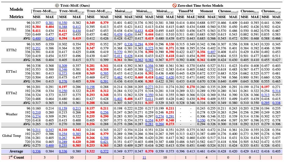
The authors evaluate all TIME-MOE variants on 2 benchmarks - containing 6 popular datasets.

1. Zero-Shot Forecasting: The model is compared to other popular zero-shot models - TimesFM (Google), MOIRAI (Salesforce), and MOMENT (Carnegie Mellon & University of Pennsylvania)

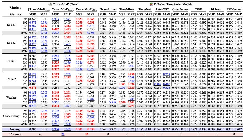
2. Full-shot Forecasting: TIME-MOE is fine-tuned for 1 epoch on the training parts of the datasets and compared to fully-tuned models like PatchTST and TiDE.

Both benchmarks use MAE and MSE as evaluation metrics. Importantly, the datasets used for benchmarking were excluded from TIME-MOE's pretraining data to ensure fair comparisons.

Let’s start with the zero-shot forecasting benchmark:

Figure 6: Comparing Time-MOE with different forecasting models in a zero-shot forecasting scenario (Image source)

We notice the following:

• Time-MOE scores the most wins across all datasets and horizons.

• MOIRAI-base achieves the best MAE score on average(closely followed by Time-MOE-ultra) and Time-MOE-ultra achieves the best MSE error.

• Interestingly, MOIRAI-base outperforms MOIRAI-large, a pattern also seen in VisionTS’s and MOIRAI’s benchmarks. This is likely due to MOIRAI-large being undertrained, as suggested by scaling laws.

• Unfortunately, Tiny Time Mixers, a powerful MLP-based foundation forecasting model, is absent from the benchmark.

Figure 7 shows the full-shot forecasting benchmark:

Figure 7: Comparing Time-MOE with different forecasting models in a full-shot forecasting scenario (Image source)

• Here, Time-MOE-ultra scores the most wins and achieves the lowest MAE and MSE scores.

• PatchTST (Transformer-based) and TimeMixer (MLP-based), both SOTA in their categories, also score some wins.

• Time-MOE-base is not very competitive, but Time-MOE-ultra is impressive - especially considering it was finetuned for 1 epoch only.

• It would be nice if that benchmark also included some extra models from other domains like Tree-based or statistical models.

Scaling Laws

I have consistently emphasized the importance of scaling laws for the success of foundation models. You can read more about them here:

VisionTS : Building High-Performance Forecasting Models from Images

The power of foundation models lies in their ability to leverage scale—how more data, longer training, and more parameters boost performance.

The Time-MOE authors explored how their model scales, benchmarking every Time-MOE variant in both sparse and dense formats:

Figure 8: Comparison of sparse and dense models regarding training and inference costs. (Left) Average MSE across 6 benchmarks, comparing TIME-MOE and dense models, both trained from scratch with varying data sizes. (Right) (Image Source)

The results are quite promising:

• Left figure: Sparse Time-MOE variants are significantly faster in training and inference, with the gap narrowing for Time-MOE-ultra. Larger models delegate input to multiple experts with greater efficiency.

• Right figure: Both sparsity and larger training datasets substantially benefit Time-MOE.

When I launched this newsletter a year ago, I argued that the success of foundation models hinges on scaling laws.

I discussed this when TimeGPT, the first foundation model, was introduced:

TimeGPT: The First Foundation Model for Time Series

It’s now clear that scaling laws benefit larger time-series models, with much potential for future research.

Time-MOE in Practice

Only the base version of the model has been released at the time of this writing. You can find the model and the dataset here. The other variants will be released shortly.

I’ve also prepared a mini-tutorial featuring the smallest model, Maple728/TimeMoE-50M, available in the AI Projects folder. For comparison, I benchmarked this model against other popular statistical models:

Image by author

The model performed well as a zero-shot forecaster. One thing I noticed is that increasing the context_length did not benefit the model (unlike other foundation models).

The authors also suggested that fine-tuning (for at least 1 epoch) may be necessary to unlock the model's full potential.

The fine-tuning code will also be released (according to the authors).

Closing Remarks

Time-MOE is a major contribution to the forecasting community, introducing innovative features. Combining Mixture-of-Experts with foundation models was only a matter of time, given the architecture's success in language models.

Currently, Time-MOE supports only univariate forecasting, but future updates may include extra features, similar to what other foundation models did. Its architecture could be easily adapted to handle covariates, by e.g. allowing SwiGLU to tokenize a vector of covariates instead of a single time point.

Shortly after Time-MOE was released, MOIRAI was also enhanced with Mixture-of-experts — showing additional improvements over vanilla MOIRAI. We’ll discuss this model next as well so stay tuned!

Thank you for reading!

Horizon AI Forecast is a reader-supported newsletter, featuring occasional bonus posts for supporters. Your support through a paid subscription would be greatly appreciated.

References

Shi et al. Time-moe: Billion-scale Time Series Foundation Models With Mixture Of Experts